Visualizing Deposit Trends Over Time

Exploring transaction data with pandas gave me a baseline. Counting things, grouping things, building a sense of what normal looks like. That was useful, but it left me staring at tables of numbers. What I wanted was to see the shape of what's happening over time.

That's where visualization comes in. Deposit competition is near the top of every community bank's worry list right now. Banks are watching their deposit base carefully, especially with rates moving. Tables of monthly totals don't make the patterns obvious. Charts do.

I'm going back to the same Berka dataset from last time, 1,056,320 transactions across 4,500 accounts. This time, instead of counting and grouping, I want to build charts that tell a story.

Getting the Data Ready

The first step is turning individual transactions into something we can chart over time. Each transaction has a running balance, so if we grab the last transaction per account per month, we get an end-of-month snapshot.

import matplotlib.pyplot as plt
import pandas as pd

tx = pd.read_csv('transaction.csv', low_memory=False)
tx['date'] = pd.to_datetime(tx['date'])
tx['month'] = tx['date'].dt.to_period('M')

# Last balance per account per month
monthly = tx.sort_values('date').groupby(
    ['account_id', 'month']
).last().reset_index()

That groupby and last() pattern is one I keep reaching for. Sort by date first, then group by account and month, and the last row in each group gives us the final balance for that period. From there, we can aggregate however we want.

Total Deposits Over Time

The first chart is the one that answers the simplest question. How much money is sitting in this bank?

total = monthly.groupby('month')['balance'].sum().reset_index()
total['month_dt'] = total['month'].dt.to_timestamp()

fig, ax = plt.subplots(figsize=(10, 5))
ax.plot(total['month_dt'], total['balance'] / 1e6,
        color='#1e3a5f', linewidth=2)
ax.fill_between(total['month_dt'], total['balance'] / 1e6,
                alpha=0.1, color='#1e3a5f')
ax.set_ylabel('Total Deposits ($M)')
ax.set_title('Total Deposits Across All Accounts')
ax.grid(True, alpha=0.3)
plt.tight_layout()
plt.savefig('total-deposits-over-time.png', dpi=150)

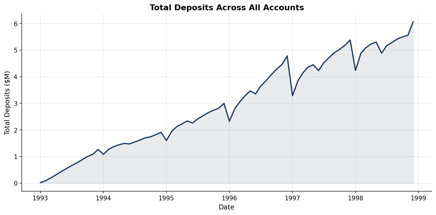
The shape is striking. Total deposits climb from almost nothing in early 1993 to over $6 million by the end of 1998. That's a steep, steady rise. But the chart alone doesn't tell us why. Is it because existing clients are saving more, or because new accounts keep opening? We'll need more charts to untangle that.

Where the Money Flows

Instead of just looking at the balance, let's separate the inflows from the outflows. Every credit transaction is money coming in, every debit or withdrawal is money going out.

credits = tx[tx['type'] == 'credit'].groupby('month')['amount'].sum()
debits = tx[tx['type'].isin(['debit', 'cash_withdrawal'])].groupby(
    'month')['amount'].sum()

flows = pd.DataFrame({
    'inflows': credits, 'outflows': debits
}).fillna(0).reset_index()
flows['month_dt'] = flows['month'].dt.to_timestamp()

fig, ax = plt.subplots(figsize=(10, 5))
ax.bar(flows['month_dt'], flows['inflows'] / 1e6,
       width=25, label='Inflows', color='#0d9488', alpha=0.8)
ax.bar(flows['month_dt'], -flows['outflows'] / 1e6,
       width=25, label='Outflows', color='#f97316', alpha=0.8)
ax.axhline(y=0, color='black', linewidth=0.5)
ax.set_ylabel('Amount ($M)')
ax.set_title('Monthly Inflows vs. Outflows')
ax.legend()
plt.tight_layout()
plt.savefig('inflows-vs-outflows.png', dpi=150)

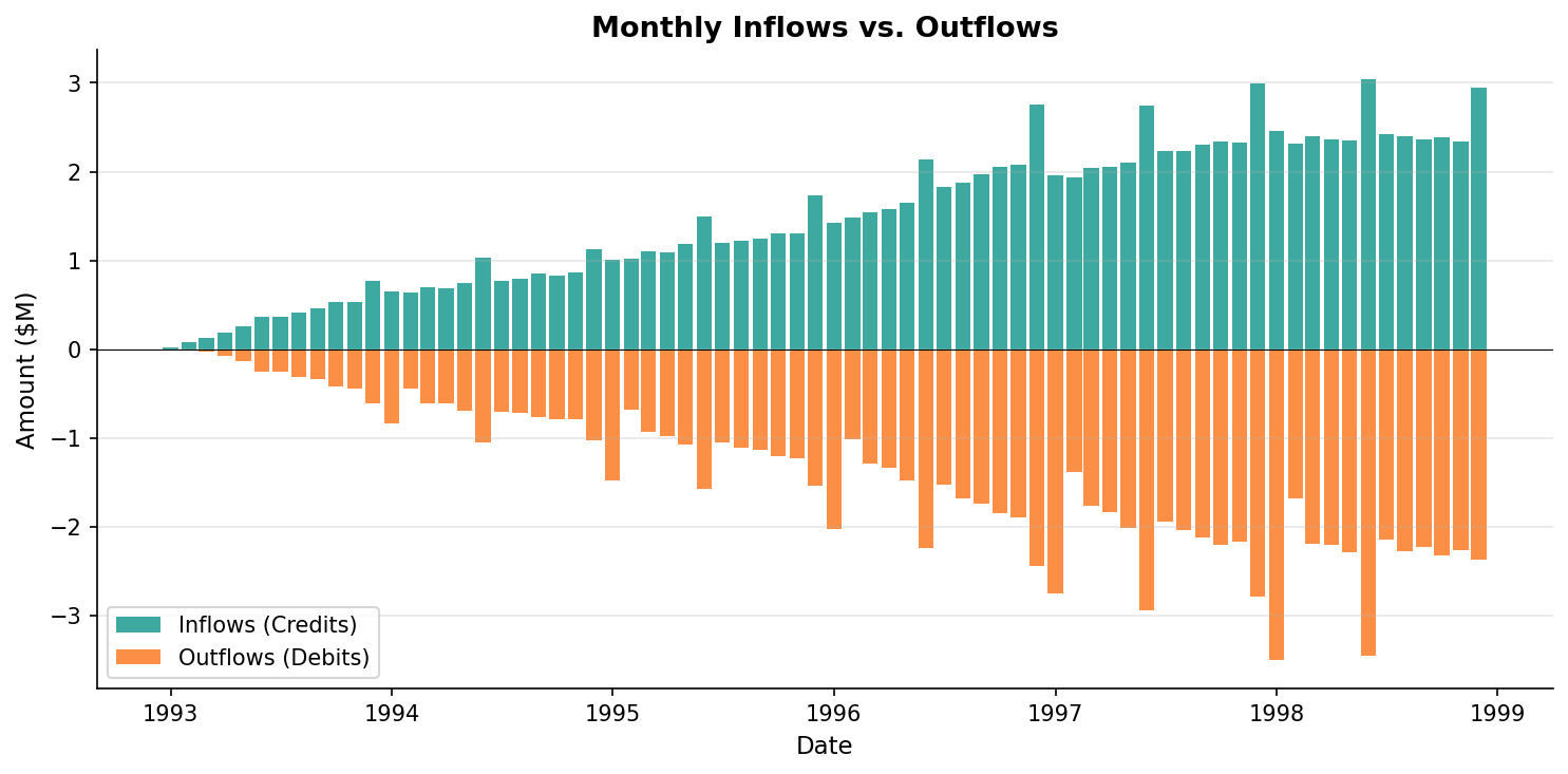
This one tells a healthier story. Average monthly inflows run about $1.5 million, outflows about $1.4 million. The net is positive in 62 out of 72 months. That consistent positive gap is what drives the upward trend in the first chart. But notice how both bars get taller over time. That's not just more money moving through existing accounts. It's more accounts generating more activity.

Average Balance vs Account Growth

The question worth asking is whether the total deposit growth is real growth or just more accounts. A dual-axis chart can separate those two things.

avg_bal = monthly.groupby('month')['balance'].mean().reset_index()
avg_bal['month_dt'] = avg_bal['month'].dt.to_timestamp()

active = monthly.groupby('month')['account_id'].nunique().reset_index()
active.columns = ['month', 'active_accounts']
active['month_dt'] = active['month'].dt.to_timestamp()

fig, ax1 = plt.subplots(figsize=(10, 5))
ax1.plot(avg_bal['month_dt'], avg_bal['balance'],
         color='#1e3a5f', linewidth=2, label='Avg Balance')
ax1.set_ylabel('Average Balance ($)', color='#1e3a5f')

ax2 = ax1.twinx()
ax2.plot(active['month_dt'], active['active_accounts'],
         color='#0d9488', linewidth=2, linestyle='--',
         label='Active Accounts')
ax2.set_ylabel('Active Accounts', color='#0d9488')

lines1, labels1 = ax1.get_legend_handles_labels()
lines2, labels2 = ax2.get_legend_handles_labels()
ax1.legend(lines1 + lines2, labels1 + labels2, loc='center left')
ax1.set_title('Average Balance vs. Active Account Count')
plt.tight_layout()
plt.savefig('avg-balance-vs-accounts.png', dpi=150)

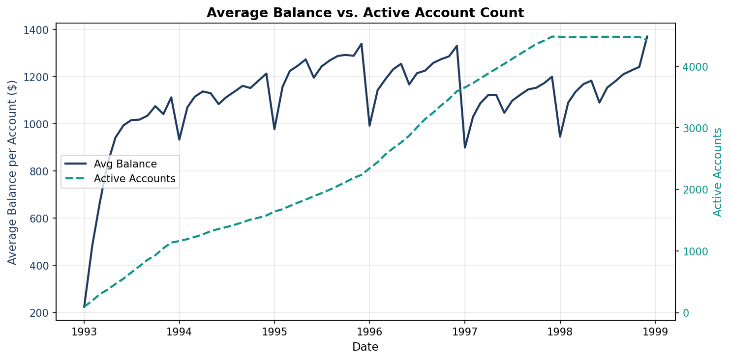
Now the picture gets interesting. Active accounts climb steadily, from under 100 to nearly 4,500, which explains most of the total deposit growth. But the average balance per account also rises, from around $200 to over $1,300. That means existing accounts are growing too, not just new ones opening. Both factors are contributing.

What the Charts Reveal

Four charts, and a much clearer picture than the tables gave us. The total deposit line looks impressive until you realize most of the growth comes from new accounts. The inflow and outflow chart shows the bank is consistently taking in more than it sends out, which is healthy. And the dual-axis chart shows that even on a per-account basis, balances are growing.

This is exactly the kind of analysis that matters for the deposit competition question. If a bank is watching its deposit base, it's not enough to track total deposits. You need to separate the drivers. Is growth coming from new relationships or deeper existing ones? Are outflows accelerating? Is the net flow shrinking even if total deposits are still climbing?

These are basic matplotlib charts with minimal styling. In a real analysis, I'd add annotations for specific events, smooth out the noise with rolling averages, maybe layer in rate data to see if deposit behavior shifts when rates move. But even these simple visualizations told me more in five minutes than the raw numbers did in an hour.