Getting Started with Jupyter Notebooks

Any real work with data starts with actually looking at it. Before reaching for a heavyweight analytics platform, the fastest way to get your hands on a dataset is a notebook running on your own machine. That personal workbench is where I do most of my exploring, and Jupyter is what powers it.

What is Jupyter?

Jupyter notebooks combine code, output, and notes in a single document. You write code in "cells," run each cell individually, and see the results immediately below. It's different from writing a script and running the whole thing. You can experiment, see what happens, adjust, and build up your analysis piece by piece.

The name comes from Julia, Python, and R, the three languages it originally supported, though Python is by far the most common. The notebook format has become the standard tool for data exploration, and for good reason. It makes iterative analysis natural.

Installation

If you're new to Python, the tutorial series covers the basics. Now we add the data tools. Open a terminal and run:

pip install jupyter pandas matplotlib

This installs Jupyter itself, pandas for working with tabular data, and matplotlib for visualization. Then launch Jupyter:

jupyter notebook

Your browser opens with a file navigator. Click "New" and select "Python 3" to create your first notebook.

Cells and Execution

A new notebook starts with an empty cell. Type some Python and press Shift+Enter to run it:

2 + 2

4

The output appears directly below. The cell stays there, and you can edit and re-run it anytime. Add a new cell below with the + button or by pressing B (for "below").

Cells can also contain markdown for notes. Change the cell type using the dropdown menu or press M. This is useful for documenting your thinking as you explore.

Pandas Basics

Pandas is a library for working with tabular data, the kind of data you'd normally see in a spreadsheet or database table. The core object is called a DataFrame, which is essentially a table with named columns.

Let's create one from scratch:

import pandas as pd

data = {
    'name': ['Checking', 'Savings', 'CD', 'Money Market'],
    'balance': [5200, 12000, 25000, 8500],
    'rate': [0.01, 0.5, 2.0, 0.75]
}

df = pd.DataFrame(data)
df

           name  balance  rate
0      Checking     5200  0.01
1       Savings    12000  0.50
2            CD    25000  2.00
3  Money Market     8500  0.75

The pd is a common alias for pandas. The DataFrame displays as a nice table with row numbers (the index) on the left.

You can access individual columns:

df['balance']

0     5200
1    12000
2    25000
3     8500
Name: balance, dtype: int64

This returns a Series, which is like a single column. You can do math on it:

df['balance'].sum()

50700

df['balance'].mean()

12675.0

Filtering is straightforward:

df[df['rate'] > 0.5]

           name  balance  rate
2            CD    25000  2.00
3  Money Market     8500  0.75

This returns only the rows where the rate is greater than 0.5.

Matplotlib Basics

Matplotlib handles visualization. The most common import pattern gives you a plt object for creating charts:

import matplotlib.pyplot as plt

df.plot(kind='bar', x='name', y='balance', color='#1e3a5f', legend=False)
plt.title('Account Balances')
plt.ylabel('Balance ($)')
plt.tight_layout()

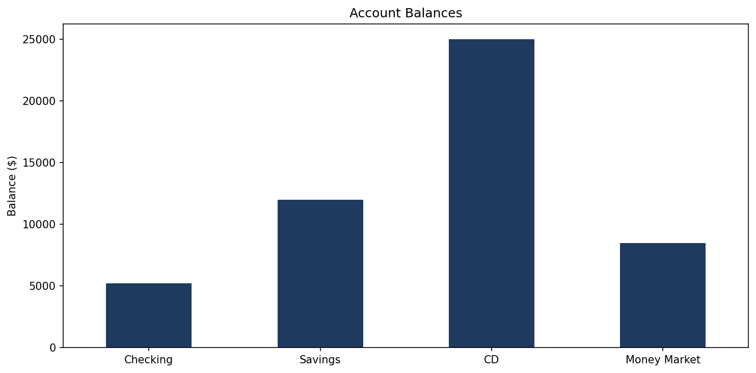
The chart appears directly in the notebook. Pandas DataFrames have a .plot() method that wraps matplotlib, making simple charts easy. For a bar chart, you specify kind='bar' and which columns to use for the x and y axes.

Line charts work similarly:

months = ['Jan', 'Feb', 'Mar', 'Apr', 'May', 'Jun']
deposits = [4200, 4800, 5100, 4900, 5300, 5600]

plt.plot(months, deposits, marker='o', color='#0d9488', linewidth=2, markersize=8)
plt.title('Monthly Deposits')
plt.ylabel('Amount ($)')
plt.tight_layout()

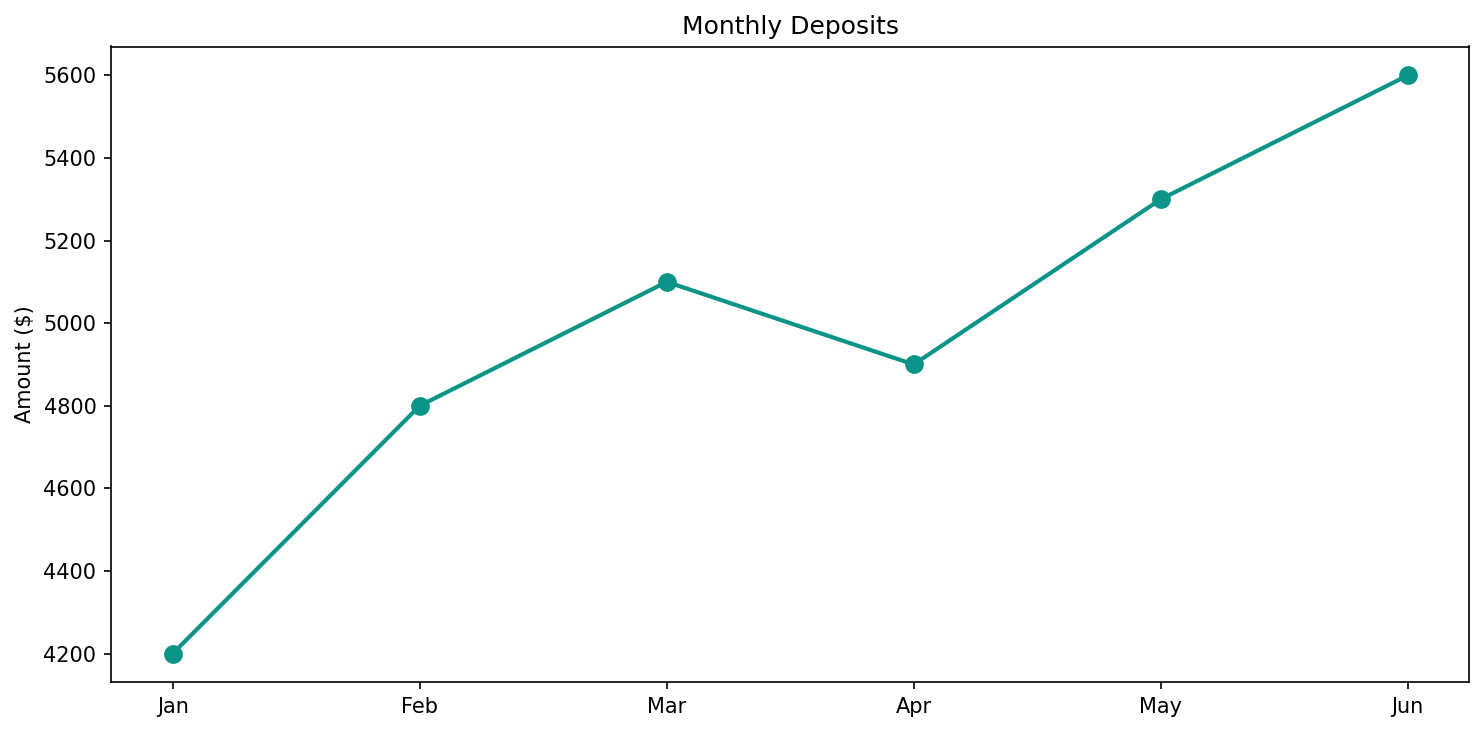
The marker='o' adds dots at each data point. You can customize colors, line styles, and add multiple lines to the same chart as your needs grow.

Loading External Data

Most real analysis starts with loading data from a file. The most common format is CSV:

df = pd.read_csv('filename.csv')

Once loaded, a few commands tell you what you're working with:

df.head()       # First 5 rows
df.info()       # Column names, types, and missing values
df.describe()   # Statistics for numeric columns
df.shape        # Number of rows and columns

These become reflexive. Every time I load a new dataset, I run these four commands first to understand what I'm dealing with.

What's Next

With Jupyter, pandas, and matplotlib set up, we have the foundation for serious data exploration. The notebook format encourages experimentation. You can try things, see results, and iterate quickly.

In the next post, we'll put these tools to work on real data, the publicly available mortgage lending records that banks are required to report. It's a chance to see how the techniques we've just covered apply to actual questions about lending patterns.